Mathematical Models for Acoustic Analysis

Standard acoustic problems involve solving for the small acoustic pressure variations p on top of the stationary background pressure p0. Mathematically this represents a linearization (small parameter expansion) around the stationary quiescent values.

The governing equations for a compressible lossless (no thermal conduction and no viscosity) fluid flow problem are the momentum equation (Euler’s equation) and the continuity equation. These are given by:

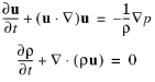
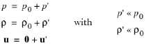
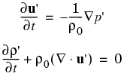
where ρ is the total density, p is the total pressure, and u is the velocity field. In classical pressure acoustics, all thermodynamic processes are assumed reversible and adiabatic, known as an isentropic process. The small parameter expansion is performed on a stationary fluid of density ρ0 (SI unit: kg/m3) and at pressure p0 (SI unit: Pa) such that:

where the primed variables represent the small acoustic variations. Inserting these into the governing equations and only retaining terms linear in the primed variables yields:

One of the dependent variables, the density, is removed by expressing it in terms of the pressure using a Taylor expansion (linearization)

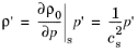
where cs is recognized as the (isentropic) speed of sound (SI unit: m/s) at constant entropy s. The subscripts s and 0 are dropped in the following.

Finally, rearranging the equations (divergence of momentum equation inserted into the continuity equation) and dropping the primes yields the wave equation for sound waves in a lossless medium

(11-1)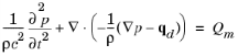

The speed of sound is related to the compressibility of the fluid where the waves are propagating. The combination ρ  c2 is called the bulk modulus, commonly denoted K (SI unit: N /m2). The equation is further extended with two optional source terms:

•	The dipole source qd (SI unit: N/m3)

•	The monopole source Qm (SI unit: 1/s2)

A special case is a time-harmonic wave, for which the pressure varies with time as

where ω = 2π   f (SI unit: rad/s)  is the angular frequency and  f (SI unit: Hz) is denoting the frequency. Assuming the same harmonic time-dependence for the source terms, the wave equation for acoustic waves reduces to an inhomogeneous Helmholtz equation

(11-2).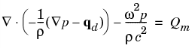

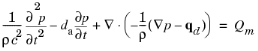
With the two source terms removed, this equation can also be treated as an eigenvalue PDE to solve for eigenmodes and eigenfrequencies.

Typical boundary conditions for the wave equation and the Helmholtz equation are:

•	Sound-hard boundaries (walls)

•	Sound-soft boundaries

•	Impedance boundary conditions

•	Radiation boundary conditions

In lossy media, an additional term of first order in the time derivative needs to be introduced to model attenuation of the sound waves

where da is the damping coefficient. Note also that even when the sound waves propagate in a lossless medium, attenuation frequently occurs by interaction with the surroundings at the boundaries of the system.