Frequency Domain Study

The frequency domain — or time-harmonic — formulation uses the following inhomogeneous Helmholtz equation:

(11-3)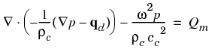

In this equation, p = p (x, ω) (the dependence on ω is henceforth not explicitly indicated). With this formulation you can compute the frequency response of a system for a number of frequencies. The default frequency domain study sets up a parametric sweep over a frequency range using a harmonic load.

When there is damping, ρc and cc are complex-valued quantities.

Equation 11-3 is the equation that the software solves for 3D geometries. In lower-dimensional and axisymmetric cases, restrictions on the coordinate dependence mean that the equations differ from case to case. Here is a brief summary of the situation.

2D

In 2D, the pressure is of the form

which, inserted in Equation 11-3, gives

(11-4)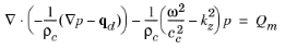

The out-of-plane wave number, kz, can be set on the Pressure Acoustics page. By default its value is 0. In the mode analysis type, −ikz is used as the eigenvalue.

2D Axisymmetry

For 2D axisymmetric geometries, the independent variables are the radial coordinate, r, and the axial coordinate, z. The only dependence allowed on the azimuthal coordinate, , is through a phase factor,

(11-5)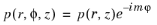

where m denotes the circumferential wave number. Because the azimuthal coordinate is periodic, m must be an integer. Just like kz in the 2D case, m can be set on the Settings window for Pressure Acoustics.

As a result of Equation 11-5, the equation to solve for the acoustic pressure in 2D axisymmetric geometries becomes

1D Axisymmetry

In 1D axisymmetric geometries,

leading to the radial equation

where both the circumferential wave number m, and the axial wave number kz, appear as parameters.

1D

The equation for the 1D case is obtained by taking the pressure to depend on a single Cartesian coordinate, x: