Component couplings establish couplings between different parts of a model component or between different model components. A component coupling is defined by a coupling operator, taking an expression as its argument when you use it (for example, to compute an average concentration). When the operator is used at a point in the destination geometry, for example, the value is computed by evaluating the argument in the source geometry. You can use a coupling operator to compute several quantities that use the same type of coupling between a source and a destination by calling it with different arguments. All types of component couplings have a source and a destination.
|
|
The source is a subset of a single model component (such as some domains or boundaries) where the coupling operator evaluates the supplied expression (as an integration over the source, for example), while the destination is the part of the geometry where the result of the coupling operator is defined. The destination can, depending on the type of coupling, be a subset of one or several model components or a “global destination” (for a scalar value that is available everywhere). The coupling operator’s value is computed by evaluating the expression given as an argument at one or several points in the source. The source and destination are both geometrical objects, but the source is limited to a single geometry, or a part of a single geometry, whereas the destination is often global.
|
•
|
|
•
|
|
•
|
Extrusion. These operators — General Extrusion, Linear Extrusion, Boundary Similarity, and Identity Mapping — connect a source and a destination and take an expression as an argument. When it is evaluated at a point in the destination, its value is computed by evaluating the argument at a corresponding point in the source. When the source and destination are of the same space dimension, it is typically a pointwise mapping. When the destination has a higher dimension than the source, the mapping is done by extruding pointwise values to the higher dimensions. For some examples of the use of extrusion coupling operators, see Examples of Extrusion Couplings.
|
|
•
|
Projection. These operators — General Projection and Linear Projection — evaluate a series of line or curve integrals on the source, where the line or curve positions depend on the positions of the evaluation points in the destination. In this way it is possible to compute the integral of an expression over one space variable for a range of different points along the other space axis, giving a result that varies over the latter space variable. For example, you can obtain the average along the y direction of a variable u defined on some 2D domain in the xy-plane by computing the integral
|
You can compare the projection couplings to creating a 2D projection as a shadow on a wall using lighting on a 3D object. COMSOL uses a method whereby it first applies a one-to-one map to the mesh of the source. It then carries out the integrals in the source over curves that correspond to vertical lines in the transformed source mesh. You can define the map between source and destination in two ways: as a linear projection or as a general projection. For some examples of the use of projection coupling operators, see Examples of Projection Couplings.
|
|
The projection coupling does not project the srcdim-dimensional source onto the destination: it projects the source onto the srcdim−1 lowest dimensions of the intermediate mesh, from which results are fetched using the destination transformation. Any domain where the destination transformation can be evaluated is a valid destination; the destination’s topology is not related to the projection process in any way, except for the constraint that the destination transformation it must map the destination points into the region of srcdim−1-dimensional space where there is any data to fetch.
|
|
•
|
Scalar. These operators — Integration, Average, Maximum and Minimum — define a scalar value such as an integration, the average over a set of geometric entities, or the maximum or minimum value of an expression and have a “global destination” (that is, they are available everywhere in the model) that you do not need to specify:
|
|
-
|
An Integration coupling operator is the value of an integral of an expression over the source, which is a set of geometric entities (domains, for example).
|
|
-
|
An Average coupling operator computes the average of an expression over the source.
|
|
-
|
A Maximum or Minimum coupling operator computes the maximum or minimum, respectively, of an expression over the source.
|
These operators can be evaluated anywhere in a model, and the value does not depend on where in the model the evaluation occurs. Integration couplings are useful for evaluating integrated quantities. To evaluate the total current across a boundary in a 2D Electric Currents model, for example, define an integration coupling operator intop1 with a source on the boundary where the current flows. Then the value of intop1(ec.normJ*ec.d), where normJ is the current density norm (SI unit: A/m2) and d is the thickness of the 2D geometry (SI unit: m), is the total current flowing across that boundary (SI unit: A). For some other examples of the use of integration coupling operators, see Examples of Integration Couplings
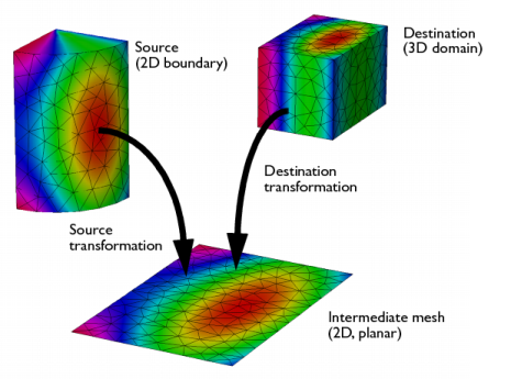
Figure 5-2: An example of a general extrusion mapping.
The definition of any extrusion coupling involves two mesh maps. The source map is a one-to-one mapping that maps the mesh of the physical source of dimension srcdim to an intermediate mesh of the same dimension embedded in a space of dimension idim ≥ srcdim. The destination map is a mapping from the destination of dimension dstdim, where the operator can be evaluated, to the same space that contains the intermediate mesh.
When the value of the coupling operator is requested somewhere in the destination, the software transforms the destination points using the destination map. It compares the resulting coordinates to the elements in the intermediate mesh to find corresponding locations in the physical source. This means that the source map must be inverted but not the destination map. The latter can in fact be noninvertible, which is, for example, the case when dstdim > idim, leading to an extrusion. If the mapping fails, select the Use NaN when mapping fails check box in the Advanced section of the Settings window for the General Extrusion and Linear Extrusion operators to evaluate the operator to NaN (Not-a-Number). Otherwise an error occurs.
|
|
All the graphics in these examples use General Extrusion component coupling.
|
 One application of a General Extrusion coupling is to mirror the solution on the x-axis. This can be useful for analysis; for example, to probe the solution at a point that is moving in time but is associated with a stationary geometry. Both source and destination are two-dimensional, as well as the intermediate mesh (srcdim = idim = dstdim). The source map is x, y (which is the default source map) and the destination map to enter is x, -y. This can also be done with a Linear Extrusion coupling operator.
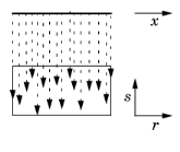 Another General Extrusion example is to extrude the solution in the 1D geometry to a 2D domain along the s-axis. The source map is x, and the destination map is r, so here srcdim = idim = 1, dstdim = 2. If the 2D geometry is Component 1 (comp1) and the 1D geometry is Component 2 (comp2), you can plot the extruded 1D solution in a 2D surface plot using comp2.genext1(u), for example, if the solution variable for the 1D solution is u.
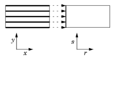
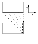 Another example maps values on the lower boundary of a rectangle that extends from x = –1 to x = 1 and from y = 0 to y = 1, to the right boundary on the same rectangle. The source map can be the default x, y and the destination map then 2*y-1, 0; alternatively, you can set the source map to x and leave the y-expression empty, and the destination map as 2*y-1 and also leave the y-expression empty. Both maps have a single component because srcdim = idim = dstdim. The difference between the first and second option is in which dimension the interpolation is performed (that is, the value of idim). The first option has the advantage that it can handle also source selections with a topology that cannot be represented in the dimension of the destination — for example, a map from a unit circle onto a line with source map x, y and destination map cos(x), sin(x). The second option has the advantage that 1D interpolation is faster and does not risk interpolation failure for coarse and non-matching meshes. This map is also linear and can be done with General Extrusion or Linear Extrusion, or with Boundary Similarity.
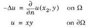
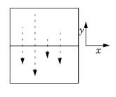
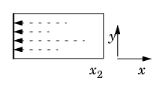
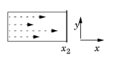 The figure to the left illustrates the extrusion process. The values of the influx on the boundary become available throughout the domain by extrusion along the y-axis. The source map is y, and the destination map is y.
|
|
All these examples use the General Projection component coupling, but they can also be done using Linear Projection component couplings.
|
 For each point r, the coupling operator returns the integral
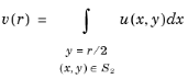
 For each point (0, s), the coupling operator returns the integral
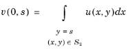
 For each point (r, 0), the coupling operator returns the integral
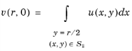
For example, if the 2D geometry is Component 1 (comp1) and the axisymmetric 2D geometry is Component 2 (comp2), you can plot the projected 2D solution in a 2D axisymmetric line plot using comp1.genproj(u), for example, if the solution variable for the planar 2D solution is u.
|
|
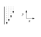
Consider the case of a single rectangular domain with Poisson’s equation. Integrate the solution squared along lines parallel to the x-axis and make the result available for analysis on the left boundary.
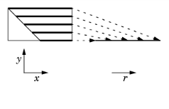
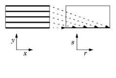
 The figure illustrates the projection process. Project the integral of the solution squared on the boundary. The source map is y, x and the destination map is y. If the projection operator is called genproj1, the desired result is obtained by evaluating genproj1(u^2).
Consider a cylinder with a radius R in the xy-plane and a height L in the z direction. For the solution u in this geometry, the following two examples describe two type of projections:
|
•
|
On one quarter of the side of this cylinder, you want to integrate the solution along curved lines of the cylinder and project it onto a straight line z = [0, L]. The source map is then z, atan2(y,x), and you leave the z-expression empty. That creates a rectangular source where the x-axis is the z-coordinate and the y-axis is the angle along the side of the cylinder, which is the direction in which you want to integrate the solution for every position along the z-axis. The destination map here is simply z (leave the y-expression empty). The integral of the solution u along the side of the cylinder is available as, for example, genproj1(u). To normalize it taking the length of the curved lines into account, use genproj1(u)/(R*pi/2) or genproj1(u)/genproj1(1), where the latter expression also gives the length of the curved lines.
|
|
•
|
It is also possible to do a projection with the cylindrical domain as the source and a boundary as target: For example, projecting the integral of u along the z-direction onto the bottom surface of the cylinder. To do so, create a General Projection coupling operator (genproj2, for example) with the default source map — x, y, z — and the default destination map: x, y. You can then plot and evaluate the projection of the integrated solution as a 2D plot on the bottom surface using genproj2(u). To get the average value, divide the projected value by the height of the cylinder using genproj2(u)/L or genproj2(u)/genproj2(1).
|
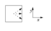 Consider Poisson’s equation on a rectangular domain. The integral of the solution squared serves as the influx in a Neumann boundary condition on the right boundary. There is a Dirichlet boundary condition on the left boundary, and the top and bottom boundaries have zero influx.
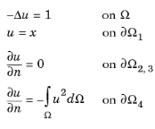
For example, define an integration coupling operator called intop1, with the rectangular domain as source. You then define the influx for the Neumann boundary condition as intop1(u^2).
 A second example is when a scalar value from a vertex is used everywhere on a boundary to which the vertex belongs. In structural mechanics you can use this type of coupling to formulate displacement constraints along a boundary in terms of the displacements of the end point. In electromagnetics the same technique can implement
 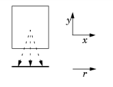 Another example is to use the integral over a domain in a 2D geometry along a domain in another 1D geometry. This approach is helpful for process-industry models where two processes interact.
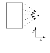 Integration coupling operators can implement integral constraints. First define a coupling operator at some vertex in such a way that it represents the value of the integral to be constrained. Then use a point constraint to set the coupling operator, and thereby the integral, to the desired value.
|
|
You can prevent the fill-in of the Jacobian matrix using the nojac operator, which forces COMSOL Multiphysics to exclude the expression that it encloses when forming the Jacobian. Using the nojac operator can slow down the convergence of the solution. Another possible solution is to add a single degree of freedom that represents the value of an expression with a scalar coupling operator.
|