Periodic Boundary Conditions

Use periodic boundary conditions to make the solution equal on two different (but usually equally shaped) boundaries.

To add a periodic boundary condition, in the Model Builder, right-click a physics interface node and select Periodic Condition. The periodic boundary condition typically implements standard periodicity so that u(x0) = u(x1) (that is, the value of the solution is the same on the periodic boundaries), but in most cases you can also choose antiperiodicity so that the solutions have opposing signs: u(x0) = −u(x1). For fluid flow physics interfaces, the Periodic Flow Condition provides a similar periodic boundary condition but without a selection of periodicity. Typically, the periodic boundary conditions determine the source and destination boundaries automatically (and display them, under Component>Definitions, in an Explicit selection node (), which is “read only”), but you can also define feasible destination boundaries manually by adding a Destination Selection subnode.

For some physics interface you can choose the direction in which you want a periodic boundary condition. For a description of the standard periodic boundary condition, which most physics interfaces use, see Periodic Condition.

The KdV Equation and Solitons: Application Library path COMSOL_Multiphysics/Equation_Based/kdv_equation.

Orientation of Source and Destination

For most periodic boundary conditions in the physics interfaces, it is possible to choose coordinate systems as a method to transform the source and destination of the periodic boundaries to an intermediate map. These settings appear in an Orientation of Source section in the main periodic condition node and in an Orientation of Destination section in an Destination Selection subnode. To display these settings, first select Advanced Physics Options from the Show menu () at the top of the Model Builder window. The possibility to specify the orientation of the periodic condition makes it possible to include twisting periodicity and periodicity between edges in shells, for example.

In both sections, there is a Transform to intermediate map list with the following options:

•

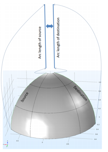
Automatic (the default). This option is only available in the Orientation of Source section in the main periodic condition node, and if selected, there is no Orientation of Destination section in an Destination Selection subnode. The automatic option relies on the geometry information to compute the arc length and the angles between two sources of the boundaries, and can be one of these methods (depending on the physics interface):

-	Automatic deduction of the periodic boundary, taking into account the rotation between source and destination. In this method, the mapping from a local coordinate on the destination to a local coordinate on the source can be written as

rdst = r − r0,dst

rsrc = rot(rdst,nsrc,ndst)

rmap = rsrc + r0,src

where nsrc and ndst are normal vectors of source and destination, respectively.

-

Automatic deduction of the periodic boundary without taking into account the rotation between source and destination. This method is useful when it is not possible to use the normal orientation to compute the rotation between source and destination. For example, on a shell or beam, the boundary selection is edges or vertices (points), but the geometry is still a 3D domain. In such cases, by neglecting the rotation, the source and the destination can be mapped via their arc lengths (see the image below).

•

Any other defined coordinate systems, one for the source and one for the destination. The Global coordinate system is always available and is the default in the Destination Selection subnode when the setting in the main periodic condition node is not Automatic. This method uses a pair of coordinate system: one is attached to source boundary, one is attached to destination boundary. Tensor transformations are used to convert components in the global system to the selected coordinate systems on the destination and source.

Periodic Boundary Condition Model Examples

In addition to the KdV Equation model example, other modules have examples using this feature:

AC/DC Module

Magnetotellurics: Application Library path: ACDC_Module/Other_Industrial_Applications/magnetotellurics

Acoustics Module

Porous Absorber: Application Library path: Acoustics_Module/Building_and_Room_Acoustics/porous_absorber

RF Module or Wave Optics Module

Fresnel Equations: Application Library path: RF_Module/Verification_Examples/fresnel_equations

Fresnel Equations: Application Library path: Wave_Optics_Module/Verification_Examples/fresnel_equations

Structural Mechanics Module

Vibrations of an Impeller: Application Library path: Structural_Mechanics_Module/Dynamics_and_Vibration/impeller