Goal-oriented error estimation is available in the Study Extensions section of the Stationary or Frequency Domain study steps.
(19-1)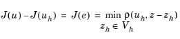
where J is a (linear) functional and the primal approximate solution  is defined by a variational formulation
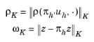
where the residual is computed by standard finite element method assembling (using numerical quadrature) for the higher-order finite-element space. This residual is then used to compute a normalized element-wise norm for each equation (here defined by the fields and their components). This technique is the same as in the mesh-adaptation algorithm (see The Adaptive Mesh Refinement Solver). Also for the error estimation, the method separates the error contribution from different equations:
where j is an equation index, and where the equations are defined from the field components.
(19-2)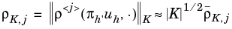
where  is the estimated maximum norm of the residual for the equation j and mesh element K. Furthermore,
(19-3)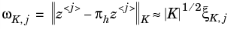
where  is the estimated maximum norm of the error for the dual solution to equation j and mesh element K. Since the exact dual solution is often not known, the weight function z − πhz must be approximated by some method. For Lagrange basis functions, the method uses the polynomial-preserving recovery technique (built-in through the ppr operator) to estimate the dual solution and thereby the error
(19-4)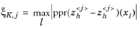
where xl are a number of coordinates in the mesh element K. These coordinates are a union of Lagrange points and Gauss points. For non-Lagrange basis functions, the polynomial-preserving recovery (PPR) technique is not supported, and the method uses a less accurate method based on the dual solution gradient and the following estimate of the dual solution error:
(19-5)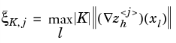
Ideally, since the error representation (Equation 19-1) is exact, the error estimate above has the potential of being very accurate. The method is not fail-safe, however. For example, the underlying PDE problem needs to be well-posed and its solution sufficiently regular. Sufficiently regular means that not only is the solution bounded in some norm, but also a number of derivatives need to be bounded in some norm. Well-posedness for the dual problem and sufficient regularity for the dual solution are also required.
|
•
|
The error estimate described here is the truncation error (also sometimes called the Galerkin error for the finite element method). It does not take into account:
|
|
-
|
The quadrature error made by using numerical methods to approximate the finite element integrals.
|
|
-
|
The geometrical approximation error made by representing the actual geometry by a polynomial representation (which is a sort of integration error for elements adjacent to or on a curved boundary).
|
|
-
|
The algebraic error obtained by terminating the solvers prematurely (or by using a sloppy tolerance).
|
|
•
|
Due to the independent maximum norms used for the dual error and the residual within each mesh element, the error estimate is normally an upper bound. When the error is very localized (to only a few elements) — for example, when a field value in a point is used as the functional — the discrepancy between the actual error and the estimated error tends to be larger than for cases where the error is less localized. For cases when the ppr method can be used, a rule-of-thumb is that the error estimate is accurate within a factor five when the error is not so localized and one order of magnitude larger when the error is very localized. When the gradient-based dual error estimation is used, the discrepancy can be much larger. This difference in accuracy occurs because this estimate does not have the correct asymptotic behavior (the correct convergence rate when the mesh size is diminished). A warning is given when the gradient method is used for a dependent variable.
|
|
•
|
The residual and dual weights (Equation 19-2 and Equation 19-3) for a component comp1.u are stored in dependent variables called comp1.res.u and comp1.dualw.u, respectively. The error variable is defined as the product of these and is accessible as comp1.err.u. These variables are accessible for plotting under Plot Group>Expression and then, for example, Component 1>Solid Mechanics>Error estimation>err.u - Error estimate u.
You can access the residual and dual weights directly through the dependent variable names. For a Stationary study step called stat (similarly for a Frequency Domain study step), the total global error is stat.errEst and the error contribution from a variable comp1.q is comp1.stat.errEst.q. The error contribution from comp1.q can be evaluated under Results>Derived Values by adding a Global Evaluation node, and then under Expression selecting Global Definitions>Error estimation>stat.errEst - Error estimate global - Stationary. The error contribution from comp1.q can be evaluated by selecting Component1>Global Definitions>Error estimation>stat.errEst.q - Error estimate q.