About the Time-Dependent Solver

	Time in the COMSOL Multiphysics Programming Reference Manual.

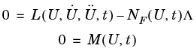
which is often referred to as the method of lines. Before solving this system, the algorithm eliminates the Lagrange multipliers Λ. If the constraints 0 = M are linear and time independent and if the constraint force Jacobian NF is constant, then the algorithm also eliminates the constraints from the system. Otherwise it keeps the constraints, leading to a differential-algebraic system.

In COMSOL Multiphysics, the IDA and generalized-a solvers are available to solve the above ODE or DAE system:

•

IDA was created at the Lawrence Livermore National Laboratory (Ref. 4) and is a modernized implementation of the DAE solver DASPK (Ref. 5), which uses variable-order variable-step-size backward differentiation formulas (BDF). Optionally, a nonlinear controller can provide more careful time-step regulation, which can reduce the thrashing of time steps that increases the number of time steps and degrades performance for highly nonlinear problems in CFD, for example. See Ref. 6 for more information about the nonlinear controller (STAB controller).

•

Generalized-α is an implicit, second-order accurate method with a parameter α or ρ∞ (0 ≤ ρ∞ ≤ 1) to control the damping of high frequencies. With ρ∞ = 1, the method has no numerical damping. For linear problems, this corresponds to the midpoint rule. ρ∞ = 0 gives the maximal numerical damping; for linear problems the highest frequency is then annihilated in one step. The method was first developed for second-order equations in structural mechanics (Ref. 8) and later extended to first-order systems (Ref. 9).

For implicit time-stepping schemes, a nonlinear solver is used to update the variables at each time step. The nonlinear solver used is controlled by the active Fully Coupled and Segregated solver subnodes. These subnodes provide much control of the nonlinear solution process: It is possible to choose the nonlinear tolerance, damping factor, how often the Jacobian is updated, and other settings such that the algorithm solves the nonlinear system more efficiently.

For the BDF (IDAS) solver there is another alternative available, and that is to use the nonlinear solver built-in IDAS. This solver is used when all the and nodes are disabled. The linear solver is in this case controlled by the active linear solver subnode.

The linearization of the above system used in the Newton iteration is

where K = −∂L/∂U is the stiffness matrix,

is the damping matrix, and

is the mass matrix. When E = 0, D is often called the mass matrix.

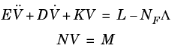
When using IDA for problems with second-order time derivatives (E ≠ 0), extra variables are internally introduced so that it is possible to form a first-order time-derivative system (this does not happen when using generalized-α because it can integrate second-order equations). The vector of extra variables, here Uv, comes with the extra equation

where U denotes the vector of original variables. This procedure expands the original ODE or DAE system to double its original size, but the linearized system is reduced to the original size with the matrix E + σ D + σ2 K, where σ is a scalar inversely proportional to the time step. By the added equation, the original variable U is therefore always a differential variable (index-0). The error test excludes the variable Uv unless consistent initialization is on, in which case the differential Uv-variables are included in the error test and the error estimation strategy applies to the algebraic Uv-variables.

For the Time-Dependent Solver under the section , the absolute and relative tolerances control the error in each integration step. More specifically, let U be the solution vector corresponding to the solution at a certain time step, and let E be the solver’s estimate of the (local) absolute error in U committed during this time step. For the , the step is accepted if

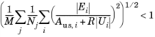
where Aus,i is the unscaled absolute tolerance for DOF i, R is the relative tolerance, M is the number of fields, and Nj is the number of degrees of freedom in field j. The numbers Aus,i are computed from a conversion of the input value Ak for the corresponding dependent variable k. For degrees of freedom for Lagrange shape functions or for ODEs, these values are the same as entered (that is, Aus,i = Ak), but for vector elements there is a field-to-DOF conversion factor involved.

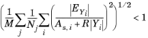
For the and when you select , the step is accepted if

where EY is the solver’s estimate of the (local) absolute error in Y, As,i is the scaled absolute tolerance for DOF i, M is the number of fields, R is the relative tolerance, Nj is the number of degrees of freedom in field j, and Yi is the scaled solution vector. For dependent variables that are using the scaling method , the numbers As,i are computed from the input values Ak according to the formula

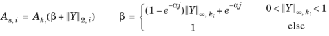
where α = 1/5, j is the time-step iteration number j = 0,1,..., and

are the 2-norm and maximum norm of the dependent variable ki , respectively. Here

is the converted input value Ak for the field k and DOF i. For dependent variables that are using another scaling method or when the check box is cleared, then

	If the solution is smaller than the absolute tolerance, there is no accuracy at all.

	For DAEs (differential-algebraic equations), you can exclude the algebraic equations from the error estimation so that the error is only based on the differential equations. See Advanced for information about excluding algebraic equations from the error estimate.

The BDF solver uses backward differentiation formulas with order of accuracy varying from one (that is, backward Euler) to five. BDF methods have been used for a long time and are known for their stability. However, they can have severe damping effects, especially the lower-order methods. Backward Euler severely damps any high frequencies. Even if you are expecting a solution with sharp gradients, you might get a very smooth solution due to the damping in the backward Euler method.

The generalized-α (alpha) solver has properties similar to the second-order BDF solver but the underlying technology is different. It contains a parameter, called α in the literature, to control the degree of damping of high frequencies. Compared to BDF (with maximum order two), generalized-α causes much less damping and is thereby more accurate. For the same reason it is also less stable.

The implementation of the generalized-α method in COMSOL Multiphysics detects which variables are first order in time and which variables are second order in time and applies the correct formulas to the variables.

In most cases, generalized-α is an accurate method with good enough stability properties. Many physics interfaces in COMSOL Multiphysics — for transport problems, for example — use generalized-α as the default transient solver. Some complicated problems, however, need the extra robustness provided by the BDF method.