where A is a square matrix, x is an unknown quantity, y is a known quantity, and k is a parameter. In general, the components of the equation depend on k. Asymptotic waveform evaluation (AWE) is a basic method based on Taylor or Padé expansions that can be used to speed up the solution of such equations for varying k significantly.
The algorithm used for the AWE solver follows the description in Section 13.4 of Ref. 16. That presentation, in turn, closely follows the original papers (Ref. 17 and Ref. 18). The general form of problems that the AWE solver is intended for is
where the dependence on k can be nonlinear. A truncated Taylor expansion of x(k) around some parameter value k0 can be written as
(19-14)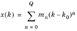
are commonly denoted moments in the literature. By repeated differentiation with respect to k and evaluation at k0, the moments can be expressed in terms of A(k0) (and derivatives thereof) and y(k0) (and derivatives thereof) as
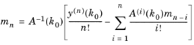
where n ≥ 1. Apparently, the linear system has to be solved for several right-hand sides. Furthermore, derivatives of A(k) and y(k) have to be computed. The moments also depend on the choice of k0, and because expansions likely have to be performed around several points, quite a few solution steps might be needed. Once the moments are available, they can be used to represent each component, xl(k), of x(k) in terms of a Padé approximations as
(19-15)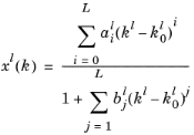
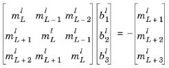
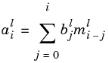
where L will be equal to 1, 2, or 3. If L = 3 and Q = 6, the bj can, via manipulations of Equation 19-14 and Equation 19-15, be seen to be the solution to
|
1
|
|
2
|
Compute expansions around fmin and fmax. Denote the approximations of
|
|
3
|