FFT Solver

The FFT Solver () performs a discrete Fourier transformation for time-dependent or frequency-dependent input solutions using FFT (fast Fourier transform). You can add the FFT solver to Time Dependent and Frequency Domain studies. The FFT solver supports both forward FFT from the time domain to the frequency domain and inverse NFT (nonuniform Fourier transform) or inverse FFT from the frequency domain to the time domain. The input solution has to be of a Time Dependent type for a forward FFT or of a Parametric type for an inverse NFT (INFT) or inverse FFT (IFFT). The input solution can have real-valued or complex-valued data. COMSOL Multiphysics uses the FFT library in Intel’s MKL for the FFT transformations in the FFT solver.

You can visualize the results of an FFT or INFT/IFFT like any other solution, and it can be postprocessed in the same way. The output is typically a complex-valued quantity. Use abs(u) to plot the absolute value, or use real(u) and imag(u) to plot the real and imaginary parts, respectively.

Forward FFT

For the forward FFT (the time-dependent case), a time-dependent solution is transformed from times {t0,…, tN−1} to frequencies {f0, …, fN−1} in the frequency domain.

Inverse NFT/Inverse FFT

For the inverse NFT or inverse FFT (the frequency domain case), a frequency-dependent solution is transformed from frequencies {f0, …, fN−1} to times {t0, …, tK−1} in the time domain. The FFT algorithm is used for the inverse transformation if the input frequency list and the output time list are equidistant and the output time range given matches the input data. Otherwise, the NFT algorithm is used.

If you have the Structural Mechanics Module, see one of these example using the FFT solver: • Vibration Analysis of a Deep Beam: Application Library path Structural_Mechanics_Module/Verification_Examples/vibrating_deep_beam • Viscoelastic Structural Damper: Application Library path Structural_Mechanics_Module/Dynamics_and_Vibration/viscoelastic_damper_frequency

General

From the Defined by study step list, select a corresponding Frequency to Time FFT or Time to Frequency FFT study step (the default if such a study step created the FFT Solver node; the FFT solver settings are then controlled from the study step), or select User defined to define the corresponding settings in the FFT solver (see below).

From the Transformation list, choose Forward for a forward FFT from the time domain to the frequency domain or Inverse for an inverse NFT/FFT from the frequency domain to the time domain. If a study step controls the FFT solver, the transformation setting is determined from that study step.

From the Solution list you can select any applicable solution, including solutions from other studies. You can also select Current, which uses the current solution. Depending on the type of solution selected, a Use list may appear where you can choose Current, to use the current solution, or a stored solution (Solution Store 1, for example).

For scaling of the solution, from the Scaling list choose Discrete Fourier transform (the default) for discrete scaling (unscaled) or Continuous Fourier transform for continuous scaling (scaled by time or frequency step).

Window Function

You can apply a window function for the input data by selecting the Use window function check box. A window function can be useful to restrict the input data. The following options are available from the Window function list:

•	Choose From expression (the default) to use a real or complex user-defined Expression. Every input value is multiplied by this expression. The expression can be parameterized using the following parameters:

-	t: the time tk in the forward FFT case.

-	freq: the frequency fk in the inverse FFT case.

-	niterFFTin, which corresponds to the index j in the forward and inverse FFT cases.

-	nFFTin: the number of input samples for the forward and inverse FFT cases (that is, 0 ≤ niterFFTin < nFFTin).

-	tPeriodFFT: the period in time for the forward FFT case; that is, t in {t0,…, tN−1} with tPeriodFFT equal to tN−t0.

-	freqmaxFFT: the frequency range for the inverse FFT case; that is, freq in {f0, …, fN−1} with freqmaxFFT equal to fN−1−f0.

•

Choose Cutoff to specify a window using a Cutoff fraction c in the interval from 0 to 1. The input values are then set to u(tj) = 0 or ω(fj) = 0 for j ≥ cN. This window function provides a sharp cutoff, which might be useful in the time domain where you know that your solution has a zero or very small amplitude at the end.

•	Choose Rectangular to use a rectangular (boxcar) window, which cuts off all input data outside of the start and end values in the Window start and Window end fields.

•	Choose Gaussian to use a Gaussian window defined by a Window center value and a Standard deviation.

•	Choose Hamming to use a Hamming window defined by a Window start value and a Window end value.

•	Choose Hanning to use a Hanning (Hann) window defined by a Window start value and a Window end value.

•	Choose Blackman to use a Blackman window defined by a Window start value and a Window end value.

•

Choose Tukey to use a Tukey window (tapered cosine window) defined by a Window start value and a Window end value. In addition, there is a tuning window parameter α, which you define in the Window parameter field (default value: 0.5). If the window parameter is set to 0, the Tukey window becomes a rectangular window; if set to 1, it becomes a Hanning (Hann) window.

For general information about window functions, see Ref. 19.

In the case of a forward FFT, for all window types except the one defined from a user-defined expression and the cutoff window, you can also specify a time unit (default: s) in the Time unit list provided for the Start time and End time fields or the Window center fields.

In the case of an inverse FFT, for all window types except the one defined from a user-defined expression and the cutoff window, you can also specify a unit (default: Hz) in the Frequency unit list.

Additional Settings for the Forward FFT

From the Time unit list, choose a time unit (default: s) to use for the times in the transformation. Specify the input time range ([tstart, tend]) for the forward FFT in the Start time (tstart) and End time (tend) fields. The number of interpolated input solutions, N, is derived from the specified maximum output frequency and appears in the solver log. Specify the maximum output frequency fmax using the Frequency unit list (default: Hz) and the Maximum output frequency field.

The input solution is padded with zeros (for tstart <  t0 and tend >  tN), if the start time or end time for the FFT exceeds the time range [t0,  tN] of the time-dependent input solution. Window functions are applied to the original data (that is, the window function is applied first, then the zero padding is added).

The FFT solver adds a warning when zero padding is applied and provides the number of zero solutions added in the log. In addition, there is a warning when the values at the boundaries t0 and tN are not zero. In such cases, apply an appropriate window function.

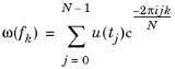
The Periodic input data check box is selected by default. The FFT solver then assumes that u(tend) = u(tstart) and performs the FFT on the values {u(t0),…, u(tN−1)} for the equidistant times t0 = tstart,…, tN−1, where tN = tend; that is, the period T is tend − tstart. The outputs are {ω(f0), …, ω(fN−1)}. The frequencies are computed by fk = k / T for k = 0, …, N−1. If you clear the Periodic input data check box, the FFT solver performs the FFT for the values {u(t0),…, u(tN−1)} for the equidistant times t0 = tstart,…,tN−1 = tend; that is, the period T is (N /( N−1))·(tend − tstart). The outputs are {ω(f0), …, ω(fN−1)}. The frequencies are computed by fk = k / T for k = 0, …, N−1. Note that the period T is different compared to the previous case. The time-dependent input solution is interpolated at the times t0…, tN−1. See the description below for information about how N is determined.

From the Store output frequencies list, choose No negative frequencies for real input (the default) or All frequencies. If you choose No negative frequencies for real input, the number of input samples N is defined by N= 2M +1, with M = floor((tend−tstart)·fmax). If you choose All frequencies, N is defined by N = M+1. In the first case, real input data is assumed and instead of ω(f0), …, ω(f2M) only ω(f0),..., ω(fM)) are stored. This is not a loss of information due to ω(fk) = ω(fk+N) = 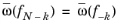(a warning is given if the input data is not real).

If you have chosen All frequencies from the Store output frequencies list, then from the Output order list, you can select Natural or Symmetric (the default):

•	If you choose Natural, the output solutions correspond to nonnegative frequency values and are ordered corresponding to ω(f0),…, ω(fN−1) or ω(f0),…, ω(fM) if the Do not store negative frequencies for real input check box is selected.

•	If you choose Symmetric the output solutions are determined for positive and negative frequencies. It results in the following output order, if the Do not store negative frequencies for real input check box is cleared:

-	ω(f−n), ω(f−(n−1)), …, ω(f−1), ω(f0), ω(f1), …, ω(fn−1), ω(fn) for N = 2n+1.

-	ω(f−n), ω(f−(n−1)), …, ω(f−1), ω(f0), ω(f1), …, ω(fn−2), ω(fn−1) for N = 2n.

The forward FFT is computed using the following unscaled formula:

for k = 0, …, N−1.

Additional Settings for the Inverse NFT/FFT

Solutions in the frequency domain are not interpolated. The input values do not have to be equidistant and they do not have to be sorted with respect to the frequencies. The input data (for nonnegative or nonpositive given frequencies) is by default extended by negative frequencies or positive frequencies with complex-conjugated input values. You can switch this behavior on and off using the Extend input samples list. Choose Add complex conjugate pairs (the default) or Use original data. The first option allows creation of real output data from complex-valued input data by basically recreating data thrown away by the Do not store negative frequencies for real input option for the forward FFT.

From the Frequencies list, select All (the default) or Select from interval:

•	For the input selection All, the inverse NFT/FFT transforms all available input solutions.

•	For the input selection Select from interval, you define the interval of frequencies using the Lower bound and Upper bound fields that appear. Choose the frequency unit from the Frequency unit list (default: Hz).

Choose the time unit from the Time unit list (default: s). Enter the output time range for the inverse NFT/FFT in the Output times field. These output times correspond precisely to the set of output time values computed. The number of output solutions can be different from the number of input solutions.

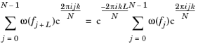
The Periodic input data check box is only available if you have selected Use original data from the Extend input samples list. The value for the highest frequency is not considered in the inverse transformation, if the Periodic input data check box is selected.

The inverse FFT is computed for input data ω(f0), …, ω(fN−1) using the following formula:

for k = 0, …, N−1. The correction factor is defined as

,

where F = fN− f0, and you can interpret it as a shift of the input values for by means of the following formula:

with ω( fj + N) = ω( fj ) for j = 0, …, N−1.

Performing an unscaled transformation (Scaling list set to Discrete Fourier Transform) means that a forward FFT times an inverse FFT results in the original input data multiplied by a factor of N. The original input is obtained if Scaling is set to Continuous Fourier Transform.

The FFT solver sorts the input data before applying the inverse FFT. For equidistant input frequencies and equidistant output, the fast transformation algorithm (FFT) is applied, if the number of input samples is equal to the number of output time values and if the given output time step (derived from the Output times list) correlates to the input frequency range.

The inverse NFT is computed using the following formula if Use original data is selected from the Extend input samples list:

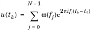
for k = 0, …, K−1 (K is given by the number of output times; that is, t0, …, tK−1. If you have selected Add complex conjugate pairs from the Extend input samples list, then the formula

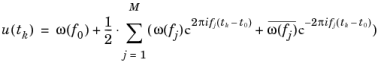
for k = 0, …, K−1 is used. The input frequencies f1, …, fM have to be all positive or all negative, and either f0 = 0 is given as input frequency or ω( f0) = 0 is used.

Select the Add stationary solution check box to extend the input data for frequency 0 by a stationary solution that is either taken as the data for frequency 0 or added to the data for frequency 0. Select the method to retrieve the solution from the Method list: Solution (the default) to use the solution itself, or Initial expression to use the expression for the initial value. Choose any available and applicable solution from the Solution list, or choose Zero for no solution. Depending on the selected solution, additional settings appear for specifying which of the solutions to use and which parameter values, eigenfrequencies, or times to use. Use the Time list to select an input solution at a specific time or to interpolate.

Advanced

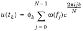
You can specify phase functions for input and output data. This functionality can be used for modifying the input and output data. Select the Use phase function check box to specify phase functions. The following options are available from the Phase function for input and Phase function for output lists: None (the default, which provides no phase function) and From expression:

Select From expression to type an expression for the phase function in the Expression field that appears. The expression ein for the input data or eout for the output data can be real valued or complex valued. In the forward case, each input value u(tk) is then multiplied by exp(i ein), and similarly, each output value ω(fk) is multiplied by exp(i eout). In the inverse case, each input value ω(fk) is multiplied by exp(i ein), and similarly, each output value u(tk) is multiplied by exp(i eout).

•	For Phase function for input, the expression ein can be parametrized using the following parameters:

-	t: the time tk in the forward FFT case.

-	freq: the frequency fk in the inverse FFT case.

-	niterFFTin, which corresponds to the index j for the input data in the forward and inverse FFT cases.

-	nFFTin: the number of input samples for the forward and inverse FFT cases.

-	tPeriodFFT: the period in time for the forward FFT case; that is, t in {t0,…, tN−1} with tPeriodFFT equal to tN−t0.

-	freqmaxFFT: the frequency range for the inverse FFT case; that is, freq in {f0, …, fN−1} with freqmaxFFT equal to fN−1−f0.

•	For Phase function for output, the expression eout can be parametrized using the following parameters:

-	freq: the frequency in the forward FFT case.

-	t: the time in the inverse FFT case.

-	niterFFTout, which corresponds to the index j for the output data in the forward and inverse FFT cases.

-	nFFTout: the number of output solutions for the forward and inverse FFT cases (that is, 0 ≤ niterFFTout < nFFTout).

-	tPeriodFFT: the period in time for the inverse FFT case; that is, t in {t0,…, tN−1} with tPeriodFFT equal to tN−1−t0.

-	freqmaxFFT: the frequency range for the forward FFT case; that is, freq in {f0, …, fN−1} with freqmaxFFT equal to fN−1−f0.

Output

The FFT solver stores temporary solution blocks on disk if you select the Store solution on disk check box. Otherwise, the temporary solution blocks are kept in memory.

Constants

In this section you can define constants that can be used as temporary constants in the solver. You can use the constants in the model or to define values for internal solver parameters. Click the Add () button to add a constant and then define its name in the Constant name column and its value (a numerical value or parameter expression) in the Constant value column. By default, any defined parameters are first added as the constant names, but you can change the names to define other constants. Click Delete () to remove the selected constant from the list.

Log

Select the Keep warnings in stored log check box if you want the warnings to remain in the log for troubleshooting or other use.