Overview

To implement a physics interface for the thermoelectric effect, you need to specify the following items:

•	The name and description for the physics interface.

•	The supported space dimension for the physics interface.

•	The study types (Stationary, Time Dependent, Eigenvalue, and so on) that the physics interface supports.

•	The equations, written using a weak formulation, to solve, and the input variables that they need.

•	The boundary conditions that the physics interface needs, including the default boundary condition, and the inputs that they need.

•	Any additional variables that are relevant to define for use in, for example, results analysis and visualization.

•	A suitable default plot to be displayed when the solver has finished and possibly custom quantities as default plot expressions for new plots.

Optionally, you can also add customized default settings for the mesh generation and the solvers.

Name and Description

The name of this interface is Thermoelectric Effect. The short name is tee. There is also a type, ThermoelectricEffect, which is primarily used by the Java® and LiveLink™ for MATLAB® interfaces.

Supported Space Dimensions

The Thermoelectric Effect interface is available in all space dimensions.

The Study Types

The Thermoelectric Effect can be made available as a Stationary and Time Dependent study types (and perhaps even other study types for more unusual applications). In this example, stationary is the only study type.

The Equations

Heat Transfer Model

The first equation is called a Heat Transfer Model and is represented by the following weak form equation:

The weak formulation using the COMSOL tensor syntax becomes

q·test(∇Τ)

In this expression, ∇ is the del vector differential operator, and · (dot) represents the dot product (scalar product).

Thermoelectric Model

The second equation is called the Thermoelectric Model and is represented by the following weak form equation:

The weak formulation using the COMSOL tensor syntax becomes

q·test(∇T)+Q*test(T)

J·test(∇V)

where * is ordinary multiplication between scalars.

A number of parameters are defined in order to efficiently use the COMSOL tensor syntax for defining the weak form equations and also variables available for results and visualization:

•	The thermal conductivity k is a user input to both the Heat Transfer Model and the Thermoelectric Model. The default value is set equal to 1.6[W/(m*K)], which corresponds to the thermoelectric material Bismuth telluride.

•	The electric conductivity σ is a second user input for the Thermoelectric Model. The default value is set equal to 1.1e5[S/m], which also corresponds to the thermoelectric material Bismuth telluride.

•	The Seebeck coefficient S is a third and final user input for the Thermoelectric Model. The default value is set equal to 200e-6[V/K], which once again corresponds to the thermoelectric material Bismuth telluride.

•	To make the definition of the weak equation easier you define a variable for the heat flux q as a 3x1 vector with the following expression:

P*J-k·∇T

There is a dot product between the thermal conductivity and the temperature gradient. This makes it easy to generalize the physics interface to an anisotropic thermal conductivity at a later time, if needed.

•	A variable for the current density J is defined as a 3x1 vector with the following expression:

-sigma·(∇V+S*∇T)

•	A variable for the Peltier coefficient P is defined as a scalar with the following expression:

S·T

•	A variable for the electric field E is defined as a 3x1 vector with the following expression:

-∇V

•	A variable for the Joule heating Q is defined as a scalar with the following expression:

J·E

The Boundary Conditions

The Thermoelectric Effect interface includes the following boundary conditions:

•	A constraint for the temperature:

T0-T

where T0 is a user input. The expression given for a constraint is understood to be set to zero, so the above constraint equation expression means: T = T0.

•	A constraint for the voltage:

V0-V

where V0 is a user input.

•	A heat flux

qin

where qin is a user input.

•	An insulation boundary condition with no user inputs. See the above theory section.

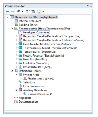
The constraint boundary conditions and the flux condition are contributing, while the insulation boundary condition is exclusive. A contributing boundary condition allows for more than one instance of the same boundary condition on a given boundary, where the model includes the combined effect of these boundary conditions. An exclusive boundary condition overrides any other previously defined boundary conditions on the given boundary. Ideally the constraint conditions should also be exclusive; however, this prevents you from having a boundary with simultaneous temperature and voltage constraints. If you accidentally set several contributing constraint boundary conditions on the same boundary, then the last boundary condition overrides all previously defined. The final Physics Builder tree displays as below: