Modeling Instructions

The following steps show how to build this model using the Thermoelectric Effect interface built in the Thermoelectric Effect Implementation section.

Model Wizard

1	Open COMSOL Multiphysics.

2	On the New page click Model Wizard () then click the 3D button () on the Select Space Dimension page.

3	On the Select Physics page under Heat Transfer>Thermoelectric Devices click Thermoelectric Effect ().

4	Click Add and then the Study button ().

5	On the Select Study page, under Preset Studies click Stationary (). Click Done ().

Geometry Modeling

1	Under Component 1 click Geometry 1 ().

2	In the Settings window for Geometry select mm from the Length unit list.

3	Add a Block () with Width 1 mm, Depth 1 mm, and Height 6 mm.

4	On the Settings window expand the Layers section. Add two layers to the table: Layer 1 with Thickness 0.1 mm and Layer 2 with Thickness 5.8 mm.

Physics Settings

1	Right-click the Thermoelectric Effect node () and select Thermoelectric Model (). This is in addition to the default node.

2	On the Settings window for the second Thermoelectric Model, add the copper electrodes (domains 1 and 3) to the selection list under Domain Selection.

3	Under Thermoelectric Model replace the defaults with the following:

-	In the Thermal conductivity field enter 350.

-	In the Electric conductivity field enter 5.9e8.

-	In the Seebeck coefficient field enter 6.5e-6.

The default Thermoelectric Model already has the correct values for bismuth telluride and is assigned to domain 2.

4	Right-click Thermoelectric Effect () and select Electric Potential ().

5	On the Settings window for Electric Potential, select boundary 3 (bottom surface) and keep the default Electric potential (0 V).

6	Right-click Thermoelectric Effect () and select Temperature ().

7	On the Settings window for Temperature select boundary 3. In the Temperature field replace the default with 273.15 K (0 degrees C).

8	Right-click Thermoelectric Effect () and select Electric Potential ().

9	On the Settings window for Electric Potential select boundary 10 (top surface). Enter an Electric potential of 0.05 V.

Mesh Generation and Computing the Solution

A mesh with default parameters is good enough for this very simple model. The default mesh is automatically created if nothing else is specified when solving.

1	Right-click the Study node and select Compute ().

Results and Visualization

The default plot under the 3D Plot Group is for the temperature T. Click the Temperature node and under Expression, replace the default Unit with degC. This is to verify the 61 degree C temperature drop.

To visualize other predefined expressions defined when creating the physics interface:

1	Under Results>3D Plot Group, click the Temperature node.

2	In the Settings window for Surface, click the Replace Expression button ().

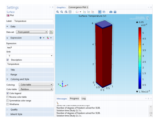
3	Under Model>Component 1>Thermoelectric Effect choose a predefined expression, for example Peltier coefficient tee.P.

4	Click the 3D Plot Group node and the Temperature plot updates in the Graphics window.