Overview

To implement a physics interface for solving Equation 4-1 above, you need to specify the following items:

•	The name and description for the physics interface.

•	The supported space dimension for the physics interface.

•	The study types (Stationary, Time Dependent, Eigenvalue, and so on) that the physics interface supports.

•	The equation, written using a weak formulation, to solve, and the input variables that it needs.

•	The boundary conditions that the physics needs, including the default boundary condition, and the inputs that they need.

•	Any additional variables that are relevant to define for use in, for example, results analysis and visualization.

•	A suitable default plot to be displayed when the solver has finished and possibly custom quantities as default plot expressions for new plots.

Name and Description

The name of this physics interface is Schrodinger Equation (avoiding using the character “ö” in the interface). The short name is scheq. There is also a type, SchrodingerEq, which is primarily used by the Java and LiveLink™ for MATLAB® interfaces.

Supported Space Dimensions

The Schrodinger Equation interface is available in all space dimensions.

The Study Types

The Schrödinger equation is an eigenvalue equation, so an eigenvalue study is the only applicable study type.

The Equation

With scalar coefficients in the equation, and using C as a replacement for the coefficient , the weak formulation using the COMSOL tensor syntax becomes

-C*∇psi·test(∇psi)-V*psi·test(psi)+lambda*psi·test(psi)

In this expression, ∇ is the nabla or del vector differential operator, and · represents an inner dot product (scalar product). * represents normal scalar multiplication. The variable lambda represents the eigenvalues (E in Equation 4-1).

The following equation parameters must be defined:

•	The reduced Planck constant, which is a predefined physical constant, hbar_const.

•	The reduced mass μ, which for a one-particle system like the hydrogen atom can be approximated as

(4-2)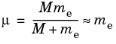

where M equals the mass of the nucleus and me represents the mass of an electron (9.1094·10−31 kg). The hydrogen nucleus consists of a single proton (more than 1800 times heavier than the electron), so the approximation of μ is valid in this case. The Schrodinger Equation interface therefore includes a user input for the reduced mass μ with a default value equal to the electron mass me, which is a predefined physical constant, me_const.

•	The potential energy V, which for a one-particle system’s potential energy is

(4-3)

where e is the electron charge (1.602·10−19 C), ε0 represents the permittivity of vacuum (8.854·10−12 F/m), and r gives the distance from the center of the atom. The Schrodinger Equation interface includes a user input for the potential energy V with a default value of 0. You can easily enter the expression above, where the electron charge e and the permittivity of vacuum ε0 are physical constants (e_const and epsilon0_const, respectively) and r is a distance that you can formulate using the space coordinates in the space dimension of the model.

The Boundary Conditions

The Schrodinger Equation interface includes the following boundary conditions:

•	Typically you assume that the exterior boundary is such that there is zero probability for the particle to be outside the specified domain. Such a zero probability boundary condition is equivalent to a Dirichlet condition Ψ = 0. This is the default boundary condition.

•	There is also a Wave Function Value boundary condition Ψ = Ψ0 for the case that you do not want to specify a zero probability. This boundary condition defines one user input for Ψ0.

•

For axisymmetric models the cylinder axis r = 0 is not a boundary in the original problem, but here it becomes one. For these boundaries the artificial Neumann boundary condition serves as an axial symmetry condition. This is the default boundary condition for axial symmetry boundaries, and COMSOL Multiphysics adds these automatically.

All boundary conditions are exclusive (that is, only one of them can be active for any of the boundaries).

Additional Variables

One variable to add is the quantity ⏐Ψ⏐2, which corresponds to the unnormalized probability density function of the electron’s position. By adding it as a variable, you can make it available as a predefined expression in plots and results evaluation.