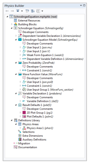
The following steps show how to define the Schrodinger Equation interface using the implementation defined in the previous section.
|
2
|
From the File menu (Windows) or the Options menu (the cross-platform version), choose Preferences. In the Preferences dialog box, select Physics Builder in the list and then select the Enable Physics Builder check box if not selected already.
|
|
3
|
From the File menu, choose New (
|
|
4
|
On the Home toolbar, click Add Physics Interface (
|
|
5
|
|
-
|
In the Description field enter Schrodinger Equation. Click the Rename node using this text button (
|
|
-
|
|
-
|
|
-
|
If you have a custom Icon for the interface, click the Browse button to locate the icon file. The default is to use the physics.png icon (
|
|
6
|
The Schrodinger Equation interface should support all space dimensions except 0D. Under Restrictions keep the defaults for the Allowed space dimensions, which already excludes 0D.
|
|
7
|
In the Allowed study types list, select the default study types (Stationary and Time dependent). Click the Add button (
|
|
8
|
In the Settings section, confirm that Domain is selected from the Top geometric entity level list. This means that the equations in the physics interface apply to the domains in the geometry, which is the case for most physics. Leave the default setting for the Default frame list as Material.
|
|
9
|
It is good practice to save the physics use interface after completing some steps. From the File menu, choose Save and create a physics interface file, SchrodingerEquation.mphphb in the default location. Click Save.
|
|
1
|
Right-click the Schrodinger Equation node and from the Variables menu select Dependent Variable Declaration (
|
|
2
|
|
-
|
|
-
|
|
-
|
|
-
|
|
-
|
|
-
|
|
3
|
In the Preferences section, both check boxes are selected by default. Keep these settings.
|
You also need to add a Dependent Variable node in the Schrödinger equation domain feature to create the shape function (element type) for the dependent variable in the domain (see Step 16 below).
|
1
|
|
2
|
|
-
|
In the Description field enter Schrodinger equation model. Click the Rename node using this text button (
|
|
-
|
|
-
|
|
3
|
In the Restrictions section, keep the default setting (Same as parent) for the Allowed space dimensions and Allow study types lists. By selecting Customized you can restrict the feature to a subset of the allowed space dimensions or study types for the physics.
|
|
4
|
In the Selection Settings section, confirm that Active is displayed in the Applicable entities list. Keep the Override rule default setting (Built in), and the Override rule default (Exclusive).
|
|
5
|
Under Coordinate Systems, keep the default settings (Frame system) for the Input base vector system and Base vector system lists. Also keep the default Frame type as Material.
|
|
6
|
Under Preferences click to select the Add as default feature check box to make this the default feature for all domains.
|
|
7
|
|
8
|
|
-
|
|
-
|
|
-
|
|
-
|
|
-
|
Keep the default settings in the Array type (Single) and Dimension (Scalar) lists for a basic scalar quantity. Also leave the Allowed values setting to Any for an entry of a general scalar number.
|
|
-
|
In the Default value field enter me_const (the electron mass, which is a built-in physical constant) in the Default value field.
|
|
9
|
This user input then becomes available as a variable schequ.mu in, for example, the predefined expressions for results evaluation. You can also refer to mu directly in the weak equation. Keep all other default settings for this node.
|
10
|
|
11
|
|
-
|
|
-
|
|
-
|
|
-
|
|
-
|
Keep the default settings in the Array type (Single) and Dimension (Scalar) lists for a basic scalar quantity. Also leave the Allowed values setting to Any for an entry of a general scalar number.
|
|
-
|
|
12
|
This user input then becomes available as a variable schequ.V in, for example, the predefined expressions for results evaluation. You can also refer to V directly in the weak equation. Keep all other default settings for this node.
|
13
|
Right-click the Schrodinger Equation Model node and from the Equations menu select Weak Form Equation (
|
|
14
|
In the Settings window locate the Integrand section. In the Expression field, enter -hbar_const^2/(2*mu)*∇psi·test(∇psi)-(V-lambda)*psi·test(psi)
|
This expression implements the Schrödinger equation formulation for this interface. Press Ctrl+Space to get a list of the supported operations that includes any special characters. See Tensor Parser for the keyboard entries to create the del operator (∇) and the dot product (·).
|
15
|
In the Selection section keep the default Selection setting (From parent), which means it inherits the selection from the top node. Also keep the default Output entities setting (Selected entities) to use the selected domains as the output. Keep all other defaults.
|
|
16
|
Right-click the Schrodinger Equation Model node and from the Variables menu select Dependent Variable Definition (
|
|
17
|
In the Settings window, locate the Definition section. From the Physical quantity list select Dimensionless (1). Lagrange elements are the most widely used and are suitable for this physics interface. The default shape-function order becomes 2. Keep the other defaults.
|
|
1
|
Right-click the Schrodinger Equation (Physics Interface 1) node and from the Features menu select Boundary Condition (
|
|
2
|
|
-
|
In the Description field enter Zero probability. Click the Rename node using this text button (
|
|
-
|
|
-
|
|
3
|
|
4
|
In the Preferences section, select the Add as default feature check box. Keep the Default entity types as Exterior to make this a default condition on exterior boundaries only.
|
|
5
|
|
6
|
In the Settings window locate the Declaration section. Enter 0-psi in the Expression field to make Ψ = 0 on the boundary (this expression is set equal to zero by the constraint).
|
|
7
|
In the Shape Declaration section, from the Physical quantity list select Dimensionless (1) to declare the correct dimension for the constrained variable Ψ. Keep all other default settings.
|
|
|
Click the Schrodinger Equation node. On the Settings window under Default Features note that the Schrodinger Equation Model and the Zero Probability boundary condition are listed.
|
|
1
|
|
2
|
|
-
|
In the Description field enter Wave function value. Click the Rename node using this text button (
|
|
-
|
|
-
|
|
3
|
|
4
|
|
5
|
|
-
|
|
-
|
|
-
|
|
-
|
|
-
|
Keep the default settings in the Array type (Single) and Dimension (Scalar) lists for a basic scalar quantity. Also leave the Allowed values setting to Any for an entry of a general scalar number.
|
|
-
|
|
6
|
|
7
|
In the Settings window locate the Declaration section. Enter par.psi0-psi in the Expression field to make Ψ = Ψ0 on the boundary. The par prefix indicates a local parameter scope and is necessary in order to refer to a user input that is not defined as a variable.
|
|
8
|
In the Shape Declaration section, from the Physical quantity list select Dimensionless (1) to declare the correct dimension for the constrained variable Ψ.
|
This feature uses a user input that should appear in a section in the Settings window. The constraint automatically adds an extra section for enabling weak constraints and set the type of constraint, but it is necessary to specify a section for the user input.
|
9
|
|
10
|
In the Settings window locate the Declaration section. In the Group name field enter WaveFunc_section and in the Description field enter Wave function.
|
|
11
|
Under the Group members list, click the Add button (
|
|
12
|
In the GUI Options section, from the GUI Layout list select Group members define a section. See User Input Group GUI Options for more information.
|
Add the probability density function ⏐Ψ⏐2 as a variable that is available in the model and for plotting (when the Show in plot menu check box is selected in the Preferences section, which is the default setting) or evaluating:
|
1
|
Right-click the Schrodinger Equation node and from the Variables menu select Variable Declaration (
|
|
2
|
|
-
|
|
-
|
|
-
|
|
-
|
|
-
|
|
3
|
Keep all the default settings in the Preferences section. The Show in plot menu check box must be selected for this variable to appear as a predefined expression in plots.
|
|
4
|
|
5
|
|
1
|
|
2
|
|
3
|
|
4
|
In the Settings window for Surface in the Description field, select the check box and enter Probability density, and then in the Expression field enter probdens.
|
|
5
|
Right-click the Surface 1 node and select Rename (or press F2). In the Rename Surface dialog box, in the New label field enter Probability Density. Click OK.
|
|
6
|
|
7
|
|
8
|
In the Settings window in the Expression field enter probdens. In the Description field enter Probability density. This makes the probability density function the default plot for all scalar plots.
|
|
1
|
|
2
|
|
-
|
|
-
|
|
-
|
The default Icon is physics.png (
|
|
-
|
In the Weight field enter 10 to make the Quantum Mechanics area appear last in the list under Mathematics (the higher the weight, the lower position the physics area gets in the tree of physics interfaces).
|
|
3
|
Under Parent Area click the Mathematics node. Click the Set as Parent button (
|
|
4
|
|
5
|
Expand the Mathematics branch and click Quantum Mechanics. Click the Set as Parent button (
|
|
6
|
Save the file that contains the physics interface as SchrodingerEquation.mphphb.
|