|
2
|
On the New page click Model Wizard (
|
|
3
|
On the Select Physics page under Mathematics>Quantum Mechanics click Schrodinger Equation (scheq) (
|
|
4
|
|
5
|
|
1
|
|
2
|
Add a Circle (
|
|
3
|
Under Position from the Base list select Center. In the r field enter 0 and in the z field enter 0, which centers the circle at the origin.
|
|
4
|
Under Rotation Angle, in the Rotation field, enter -90 degrees to create a semicircle in the right half-plane.
|
|
5
|
Click Geometry 1, and add a Circle (
|
|
6
|
Under Position from the Base list select Center. In the r field enter 0 and in the z field enter 0, which centers the circle at the origin.
|
|
7
|
Under Rotation Angle, in the Rotation field, enter -90 degrees to create a semicircle in the right half-plane.
|
|
8
|
|
1
|
Click the Schrodinger Equation Model node. In the Settings window the default in the Reduced mass field is the electron mass, me.
|
|
2
|
In the Potential energy field enter the following expression:
|
where e_const and epsilon0_const are built-in physical constants for the electron charge and the permittivity of vacuum, respectively. sqrt(r^2+z^2) is the distance r from the origin. This expression is the potential energy in Equation 4-3.
|
3
|
Verify that the default boundary conditions are correct. Click the Axial Symmetry node and confirm it applies to the symmetry boundaries at r = 0. Click the Zero Probability node to confirm it applies to the exterior boundaries of the geometry.
|
|
1
|
Right-click the Mesh node (
|
|
2
|
|
3
|
|
4
|
|
5
|
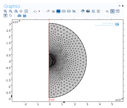
In the Element Size Parameters section, select the Maximum element size check box and enter 0.05e-9 in the corresponding field to use a mesh size no larger than 0.05 nm in domain 2.
|
|
6
|
Right-click the Mesh node (
|
|
7
|
Click the top Size node. In its Settings window click to expand the Element Size Parameters section.
|
|
8
|
In the Maximum element growth rate field replace the default with 1.1 to make the mesh size grow more slowly toward the perimeter of the geometry.
|
|
9
|
|
1
|
|
2
|
|
-
|
|
-
|
|
3
|
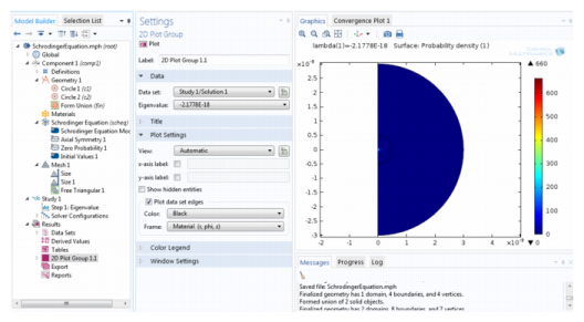
By default, COMSOL Multiphysics shows a surface plot of the probability density function ⏐Ψ⏐2 for the first eigenmode. In the Settings window for the Probability Density plot, you can also click the Replace Expression button ( ) and select Schrodinger Equation>Wave function (psi) to plot the variable psi, which is the complex-valued wave function for the electron position.
In the Settings window for the 2D Plot Group 1, you can select which eigenmode to plot. Under Data, select the corresponding eigenvalue from the Eigenvalue list. You can also verify that the eigenvalues correspond to the first energy eigenvalues listed in Results.