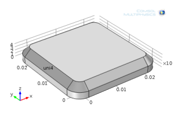
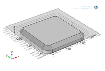
Figure 7-11 shows the geometry of a heat sink used for cooling microprocessors. The following sections describe the steps to create this geometry and introduces 3D drawing tools and techniques.
|
|
See Toolbars and Keyboard Shortcuts for links and information about all the available toolbars. Also see The COMSOL Desktop Menus and Toolbars.
It is also useful to review Working with Geometric Entities and Named Selections before continuing with these instructions.
|
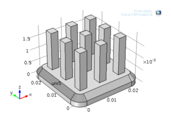
Figure 7-11: Example of a 3D heat sink geometry.
|
1
|
Double-click the COMSOL Multiphysics icon to launch COMSOL.
|
|
2
|
|
1
|
|
2
|
|
|
|
1
|
|
2
|
|
3
|
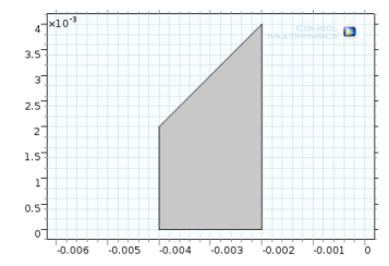
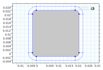
Under the Work Plane 1 node, right-click Plane Geometry and add a Bézier Polygon (
|
|
4
|
|
5
|
Under Control points: In row 1, enter -2e-3 in the xw field, and in row 2, enter −4e-3 in the xw field.
|
|
6
|
Click Add Linear to add Segment 2 (linear) to the Added segments list. Some of the Control points are automatically filled in with values; the control points from the previous line are already filled in as the starting points for the next line.
|
|
7
|
|
8
|
|
9
|
|
10
|
|
11
|
|
12
|
|
1
|
|
2
|
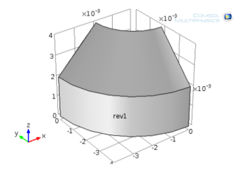
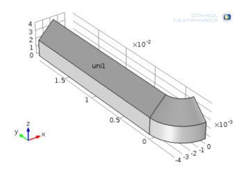
On the Settings window for Revolve under Revolution Angles, enter 90 in the End angle field (replace the default).
|
|
|
The Revolution Axis corresponds to the position of the y-axis in the work plane’s 2D coordinate system.
|
|
3
|
Under General, click to clear the Unite with input objects check box. Work Plane 1 is required for the next steps.
|
|
4
|
|
1
|
|
2
|
|
3
|
|
4
|
|
5
|
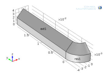
In the Graphics window click to select the objects rev1 and ext1 and add them to the Input objects section.
|
|
6
|
On the Settings window under Union, click to clear the Keep interior boundaries check box to remove the interior boundary between the corner section and the edge section.
|
|
7
|
|
1
|
|
2
|
|
3
|
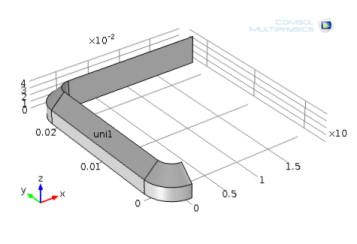
Select the Keep input objects check box to leave the input object intact as a rotation of the object is created.
|
|
4
|
|
5
|
|
6
|
|
1
|
|
2
|
In the Graphics window click to select the objects uni1 and rot1 and add them to the Input objects section under Union.
|
|
3
|
Click to clear the Keep interior boundaries check box.
|
|
4
|
|
1
|
|
2
|
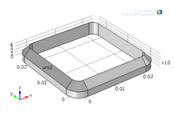
In the Graphics window click to select the object uni2 and add it to the Input objects section under Input.
|
|
3
|
|
4
|
|
5
|
|
6
|
|
1
|
|
2
|
In the Graphics window click to select the objects uni2 and rot2 and add them to the Input objects section under Union.
|
|
3
|
Click to clear the Keep interior boundaries check box.
|
|
4
|
|
1
|
|
2
|
|
3
|
On the Settings window for Work Plane 2 in the upper-left corner, click the Show Work Plane button (
|
|
4
|
|
5
|
|
6
|
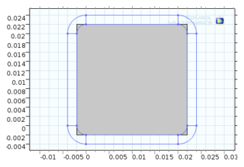
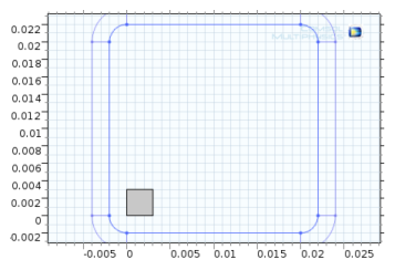
Under Position, select Center from the Base list. Then in the xw field, enter 1e-2, and in the yw field, enter 1e-2.
|
|
7
|
|
1
|
|
2
|
|
3
|
In the Graphics window click to add points 1, 2, 3, and 4 on the object sq1 to the Vertices to fillet section under Points.
|
|
4
|
|
5
|
|
1
|
|
2
|
|
3
|
|
4
|
|
5
|
On the Graphics window click to select the objects uni3 and ext2 to add to the Input objects section.
|
|
6
|
|
1
|
|
2
|
|
3
|
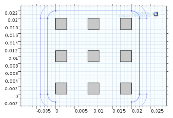
Click the Plane Geometry node under Work Plane 3. In the Settings window, the check boxes Coincident entities, Intersection, and Projection are selected by default. This visualizes the projected edges of the heat sink’s base in the work plane.
|
|
4
|
|
5
|
|
6
|
|
7
|
|
8
|
|
1
|
Under Work Plane 3 click Plane Geometry. On the Work Plane toolbar, from the Transforms menu, select Array (
|
|
2
|
|
3
|
|
4
|
|
5
|
|
1
|
|
2
|
|
3
|
|
4
|
|
5
|
On the Graphics toolbar click the Select All button (
|
|
6
|
|
1
|
|
2
|
On the Settings window under Parameters enter the following settings in the table. Replace the previous data:
|
|
3
|
|
4
|
Click the Build All button (
|